
WBCHSE Class 11 Chemistry Notes On Bohr’s Atomic Model
It was Niels Bohr, a Danish physicist, who found a way to solve the problem created by Rutherford’s model. He did not reject the nuclear model since it tallied with a-scattering experimental results.
- He tried to modify the model to account for the fact that in reality, the revolving electrons do not continuously emit radiation. He toyed with the idea that there must be some special orbits along which an electron can revolve without emitting radiation though it is constantly accelerating (i.e., changing direction).
- It is not necessary or possible (at this stage) to go into the details of how he worked out his model, but it is necessary to know its salient features. It was another of those marvelous ideas that have, from time to time, given science a big push forward.
- This was a golden era, with Planck’s quanta of energy, Einstein’s photoelectrons, Bohr’s atomic model, and other brilliant contributions that you will learn about later. For the moment, let us go back to Bohr’s model proposed in 1913, in which the electrons revolved around the nucleus according to the following rules.

Read and Learn More WBCHSE For Class11 Basic Chemistry Notes
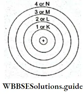
1. Electrons move around the nucleus only along certain select circular orbits, associated with definite energies. They do not revolve around any arbitrary orbit. These select orbits are also referred to as energy shells or energy levels.
| Class 11 Biology | Class 11 Chemistry |
| Class 11 Chemistry | Class 11 Physics |
| Class 11 Biology MCQs | Class 11 Physics MCQs |
| Class 11 Biology | Class 11 Physics Notes |
“WBCHSE Class 11 Chemistry, Bohr’s atomic model, and its limitations, notes”
The shells are numbered 1, 2, 3,…, or called K, L, M,… Bohr’s model, thus, utilized the concept of quantization of energy—a concept introduced by Planck and used by Einstein to explain photo electricity.
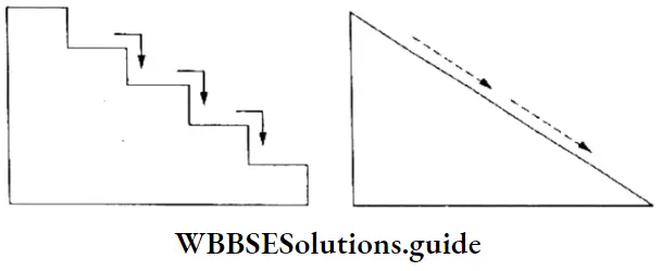
- Simply put, the quantization of a physical quantity (like energy) means that it can have only certain specific values, it cannot vary continuously to have any arbitrary value. If it changes, it can do so only discontinuously to take on particular values.
- When you go to the market to buy bananas, for example, you can buy 6, or 12, or some whole number of bananas. You cannot buy 3.25 or 5.16 bananas. In a way, the number of bananas you can buy is quantized. If this is not clear to you, consider the example illustrated in Figure.
2. As long as an electron revolves in a particular orbit or shell, it neither absorbs nor emits energy. In other words, the energy of an electron is constant in a particular orbit. This is why an orbit is referred to as a stationary state. It is a stationary state in terms of energy.
“Bohr’s atomic model, WBCHSE Class 11, chemistry notes, and key postulates”
3. The orbits an electron is permitted to move in are not only defined in terms of energy but also angular momentum. If an electron moves in a circular orbit, it will naturally have some angular momentum. Just as it can move along only select orbits associated with definite energies, it can only have specific angular momentums. The angular momentum of an electron can only be whole number multiples of h/2π, where h is the Planck constant.
Limitations Of Bohr’s Atomic Model
- Angular momentum \(\left(m_{\mathrm{e}} v r\right)=n \frac{h}{2 \pi}\), where me is the mass of the electron, v is its linear velocity, r is the radius of the circular path around the nucleus in which the electron is moving and n = 1,2,3…..
- Thus, just as the energy of an electron is quantized, its angular momentum is quantized. In other words, the energy and position of an electron in an atom are quantized.
Class 11 WBCHSE Chemistry Notes On Bohr’s Postulates And Drawbacks
4. When energy is supplied by some external source to an electron (moving in a particular stationary orbit) it may jump to a higher energy level (orbit) by absorbing a definite amount of energy. The amount of energy absorbed by the electron is equal to the difference in the energies of the higher energy level and its original (ground state) energy level.
ΔE = E2 – E1
where, ΔE = energy absorbed,
E2 = energy of higher level, and
E1 = energy of original or ground state.
- When an electron jumps to a higher energy level by absorbing a particular amount (quantum) of energy, it becomes unstable. It stays at the higher energy level only for a short while before returning to its ground state or original energy level.
- It does so by radiating the amount (photon, quantum) of energy it has absorbed to become excited or to jump to a higher level. An electron does not always jump back to the ground state by radiating the energy it has absorbed in one packet. It may radiate the energy in smaller packets, or several steps. The amount of energy it may radiate in one step, however, is quantized.
“WBCHSE Class 11, chemistry notes, on Bohr’s model, assumptions, and energy levels”
The success of Bohr’s model: Bohr was awarded the Nobel Prize in Physics in 1922. His model was a breakthrough in understanding the atomic structure. It could explain several things that Rutherford’s model could not account for.
1. It could explain why an electron does not emit radiation continuously though it is in a constant state of acceleration. In other words, it could account for the stability of the atom, which Rutherford’s model could not. (Remember, according to Bohr, an electron does not lose energy as long as it revolves in a particular stationary orbit.)
Limitations Of Bohr’s Atomic Model
2. Bohr’s theory could be used to calculate the energy of an electron in a particular orbit of the hydrogen atom (it was not valid for atoms with more than one electron, but we will come to that later).
The details of the mathematical derivation are not required here, but it can be shown that the energy of an electron in the nth orbit of the hydrogen atom works out to
\(E_n=-\frac{2 \pi^2 m e^4}{n^2 h^2}\)where m = mass of electron,
e = charge on electron,
n = number of orbits,
h = Planck constant.
Substituting the values of m,e, and h, the equation works out to be
⇒ \(E_n=-\frac{218 \times 10^{-18} \times \mathrm{Z}^2}{n^2} \mathrm{~J}\)
or, \(E_n=-\frac{1312 \times \mathrm{Z}^2}{n^2} \mathrm{~kJ} \mathrm{~mol}^{-1}\)
“Bohr’s atomic model, definition, postulates, and limitations, WBCHSE syllabus”
This formula can be used for the hydrogen atom and hydrogenlike ions, i.e., ions that have only one electron, for example, He+, Li2+, and Be3+. For He2+,
⇒ \(E_n=-\frac{4 \times 1312}{n^2} \mathrm{~kJ} \mathrm{~mol}^{-1}\)
You may wonder why the expression for the energy of an electron in the nth orbit carries a negative sign.
WBCHSE Class 11 Chemistry Notes On Bohr’s Atomic Model
Limitations Of Bohr’s Model Class 11
- This is because it is assumed that when the electron is at an infinite distance from the nucleus (i.e. when the atom is ionized and there is no force of attraction between the electron and the nucleus) its energy is zero. As the electron approaches the nucleus and enters its field of attraction, it loses energy and the atom becomes more stable.
- This is why the energy of an electron in the nth orbit is negative. By the same logic, the closer the electron gets to the nucleus, the more negative its energy becomes, or an electron in the n +1 energy level has more energy than an electron in the nth level because the nth level is closer to the nucleus than the n +1 level. The electron in the n =1 orbit has the lowest possible energy as it is closest to the positive charge of the nucleus.
Another way of looking at it is that if we wish to ionize hydrogen atoms, i.e., take the electrons from the ground state (n = 1) to infinity, we will have to supply + 1312 kJ mol -1 of energy (in this case Z =1 and n =1).
Bohr radius The radius of stationary orbitals can be calculated from the expression: \(r_n=0.529 AA\left(n^2\right)\) where n =1,2,3,…
The radius of the first stationary state is called the Bohr radius, which Is \(0.529\left(1^2\right) AA=0.529 AA\) = 52.9 pm (\(1 AA=10^{-10} \mathrm{~m}\)).
The radius of the second orbit is \(0.529\left(2^2\right) AA=2.12 AA=212 \mathrm{pm}\).
As n increases rn also increases due to the increasing distance between the nucleus and the orbit. For atoms like the hydrogen atom (containing one electron), the expression for the radius of the orbit is given by
⇒ \(r_n=\frac{0.529 AA\left(n^2\right)}{Z}\)
where Z is the atomic number. Thus, with the increase of Z, the radius becomes smaller, which means that the electron will be tightly bound to the nucleus.
3. Bohr’s model could also explain the line spectrum of hydrogen. According to his theory, an electron in the ground state (lowest possible energy level) does not emit radiation. It can, however, absorb a definite amount of energy from an external source and jump to a higher energy level, when it is said to be excited.
“Bohr’s atomic model, definition, postulates, and limitations, WBCHSE syllabus
The electron cannot remain in an excited state for long. It returns to the ground state by emitting the energy it has absorbed in the form of radiation. The frequency of the radiation emitted by the electron depends upon the difference between the energies of the two energy levels.
⇒ \(E_2-E_1=h v\)
∴ v = \(\frac{E_2-E_1}{h}\).
If E2 is the energy of the electron in the n = n2 orbit and E2 that in the n = n1 orbit then
⇒ \(v=\frac{E_{n_2}-E_{n_1}}{h}\)
⇒ \(E_{n_2}=\frac{\left(-2.18 \times 10^{-18}\right)}{n_2^2} \mathrm{~J}\)
and \(E_{n_1}=\frac{\left(-2.18 \times 10^{-18}\right)}{n_1^2} \mathrm{~J}\).
Substituting the values in the equation v = (E2- E1)/h, we get
Limitations Of Bohr’s Model Class 11
⇒ \(\mathrm{v}=\left(\frac{\left(2.18 \times 10^{-18}\right.}{6.626 \times 10^{-34}}\right)\left(\frac{1}{n_1^2}-\frac{1}{n_2^2}\right) \mathrm{s}^{-1} \quad\left(because h=6.626 \times 10^{-34} \mathrm{Js}\right)\)
⇒ \(\mathrm{v}=\left(3.29 \times 10^{15}\right)\left(\frac{1}{n_1^2}-\frac{1}{n_2^2}\right) \mathrm{s}^{-1}\).
In terms of wave number (v), we have
⇒ \(\overline{\mathrm{v}}=\frac{\mathrm{v}}{c}=\frac{3.29 \times 10^{15} \mathrm{~s}^{-1}}{3 \times 10^{10} \mathrm{~cm} \mathrm{~s}^{-1}}\left(\frac{1}{n_1^2}-\frac{1}{n_2^2}\right)\)
⇒ \(\overline{\mathrm{v}}=109,677\left(\frac{1}{n_1^2}-\frac{1}{n_2^2}\right) \mathrm{cm}^{-1}\).
Since an electron can only have certain definite energies, the energy difference between these energy levels can also only have definite values. Consequently, the frequencies of the radiations an electron emits while jumping from a higher energy level to a lower energy level will also have certain definite values. This explains why the hydrogen spectrum consists of discrete lines and is not a continuous spectrum.
“Bohr’s atomic model, WBCHSE Class 11, solved examples, and real-world applications
4. Bohr’s model thus can explain the line spectrum of hydrogen, but how does it account for the fact that the hydrogen spectrum has so many lines and that too, in different regions of the electromagnetic spectrum? What happens is that when energy is supplied to hydrogen gas the electrons of all the atoms do not absorb the same amount of energy.
- Different electrons absorb different quanta of energy to jump to different energy levels. An electron in the first shell (K) may jump to the second shell (L), or the third shell (M), and so on. When these excited electrons return to the ground state they may do so in one step (from M to K) or more than one step (from M to L and then from L to K).
- The frequency of the radiation emitted by an excited electron depends on the kind of jump or transition it makes. This accounts for the various lines in the hydrogen spectrum.
The lines in the Lyman series correspond to transitions from higher energy levels to the first energy level. Similarly, the Balmer, Paschen, Brackett, and Pfund series correspond to transitions (from higher levels) to the second, third, fourth, and fifth energy levels respectively.
WBCHSE Chemistry Notes On Bohr Model vs Quantum Mechanical Model
Example 1. According to Bohr’s model, what would be the wavelength of radiation emitted by an electron in a hydrogen atom making a transition from the fourth energy level to the first energy level?
Solution:
Energy of electron in nth orbit (En) = \(-\frac{1312}{n^2} \mathrm{~kJ} \mathrm{~mol}^{-1}\).
∴ energy of electron in fourth orbit(E1) = \(-\frac{1312}{1^2} \mathrm{~kJ} \mathrm{~mol}^{-1}\)
And energy of electron in fourth orbit (E4) = \(-\frac{1312}{4^2} \mathrm{~kJ} \mathrm{~mol}^{-1}\)
“WBCHSE Class 11 Chemistry, Bohr’s model, quantization of energy, and spectral lines”
∴ \(\quad \Delta E=E_4-E_1=-1312\left(\frac{1}{4^2}-\frac{1}{1^2}\right)\)
= \(1230 \mathrm{~kJ} \mathrm{~mol}^{-1} \text {. }\)
∴ \(\Delta E \text { per atom }=\frac{1230 \mathrm{~kJ} \mathrm{~mol}^{-1}}{\text { the Avogadro constant }}=\frac{1230 \mathrm{~kJ} \mathrm{~mol}^{-1}}{6.022 \times 10^{23} \mathrm{~mol}^{-1}}\)
= \(2.04 \times 10^{-21} \mathrm{~kJ}=2.04 \times 10^{-18} \mathrm{~J} \text {. }\)
∴ \(\Delta E=h v=h \frac{c}{\lambda}\)
∴ \(\quad \lambda=\frac{h c}{\Delta E}=\frac{6.626 \times 10^{-34} \mathrm{~J} \mathrm{~s} \times 3 \times 10^8 \mathrm{~m} \mathrm{~s}^{-1}}{2.04 \times 10^{-18} \mathrm{~J}}=9.7 \times 10^{-8} \mathrm{~m}\)
or, \(\lambda=97 \mathrm{~nm} \text {. }\)
Example 2. The ionization energy of the hydrogen atom is 13.6 eV. What will be the ionization energy of the Li2+ ion?
Solution:
Given
The ionization energy of the hydrogen atom is 13.6 eV.
The ionization energy or the energy required to remove an electron from its ground state to infinity is
∴ ionisation energy of \(\mathrm{Li}^{2+}=\frac{Z^2 E_{\mathrm{H}}}{n^2}\)
= \(\frac{(3)^2 \times 13.6}{1^2}=1224 \mathrm{eV}\)
where Z = atomic number of Li,
Eh = ionization energy of hydrogen, and
n = number of orbit = 1.
“WBCHSE Class 11 Chemistry, Bohr’s atomic model, improvements, and need for quantum mechanics”
Limitations of Bohr’s model: Bohr’s model of the atom was a great leap forward, but it by no means provided the complete picture, as scientists soon realized. It was very successful in explaining the spectrum and ionization energy of the hydrogen atom, but even with several refinements, it could not account for the spectra of atoms with more than one electron.
- Nor could it explain how molecules are formed and why they have particular shapes. Its predictions about orbital radii and velocities were also not supported by experimental results.
- A Dutch physicist, Pieter Zeeman, found that if a source emitting line spectrum is placed in a magnetic field, the spectral lines split up into finer lines. A similar thing happens when the source is placed in an electric field.
- This was discovered by the German physicist Johannes Stark. The splitting up of spectral lines in a magnetic field is called the Zeeman effect and the splitting up of the lines in an electric field is called the Stark effect. Neither of these could be accounted for by Bohr’s model. Let us summarise the difficulties Bohr’s model ran into.
- It could not account for the spectra of multi-electron atoms. Besides, the development of more sophisticated spectroscopes made it evident that each line in the hydrogen spectrum is made up of several fine lines (called fine structure), Bohr’s model could not account for this either.
- Bohr’s model could not explain the shapes of molecules or how they were formed.
- It could not explain the Zeeman effect and the Stark effect.
- The predictions made about atomic radii, velocities, etc., were not borne out by experiments.
Despite its drawbacks, Bohr’s model made a major contribution—it showed that quantum restrictions had to be applied to understand the structure of the atom.
Dual Nature Of Matter
Inspired by the dual nature of light (a concept introduced by Planck and Einstein), a French physicist, Prince Louis de Broglie, made a bold suggestion in 1924. He said that matter in general, and electrons in particular, may also have a dual nature.
To be more precise all material particles in motion have a dual behavior. This was another of those flashes of insight that we have already discussed. Louis de Broglie’s hypothesis came about a decade after Bohr’s model of the atom and almost two decades after it was established by Einstein in 1905 that light has a dual nature.
An expression for the wavelength (λ) of the wave associated with a particle of mass (m), moving with a velocity (v) was deduced by the Broglie and it is now generally known as the de Broglie equation.
∴ \(\lambda=\frac{h}{p}=\frac{h}{m v}\)
“Bohr’s atomic model, success, drawbacks, and failure to explain multi-electron atoms, WBCHSE notes”
where p = momentum of particle, and
h = the Planck constant.
This relationship implies that the wavelength of a particle in motion is inversely proportional to its momentum. It will interest you to know that most of these brilliant ideas received recognition in the form of Nobel prizes, de Broglie received the Nobel prize in 1929.
Example 1. Calculate the wavelength of a body of mass 1 mg moving with a velocity of 100 m s-1.
Solution:
Applying the de Broglie equation
∴ \(\lambda=\frac{h}{m v},\)
∴ \(\lambda=\frac{6.626 \times 10^{-34} \mathrm{~kg} \mathrm{~m}^2 \mathrm{~s}^{-1}}{1 \times 10^{-6} \mathrm{~kg} \times 100 \mathrm{~m} \mathrm{~s}^{-1}}=6.626 \times 10^{-30} \mathrm{~m}\).
Example 2. A moving electron has 5 x 10-25 J Of kinetic energy. What is its de Broglie wavelength (mass of electron = 9.1 x 10⁻³¹ kg).
Solution:
Given
A moving electron has 5 x 10-25 J Of kinetic energy.
Mass of electron = 9.1 x 10⁻³¹ kg
Kinetic energy = \(\frac{1}{2} m v^2=5 \times 10^{-25} \mathrm{~J}\)
∴ \(\quad v =\sqrt{\frac{2 \times \mathrm{KE}}{m}}\)= \(=\sqrt{\frac{2 \times 5 \times 10^{25}J}{9.1 \times 10^{-31} \mathrm{~kg}}}\)
= \(1.048 \times 10^3 \mathrm{~m} \mathrm{~s}^{-1}\)
∴ \(\quad \lambda=\frac{h}{m v}=\frac{6.62 \times 10^{-34} \mathrm{~kg} \mathrm{~m}^2 \mathrm{~s}^{-1}}{9.1 \times 10^{-31} \mathrm{~kg} \times 1048 \times 10^3 \mathrm{~m} \mathrm{~s}^{-1}}\)
= \(6.94 \times 10^{-7} \mathrm{~m}\).
“WBCHSE Class 11, chemistry notes, on Bohr’s atomic model, hydrogen spectrum, and electron orbits”
Example 3. A and D are two particles in motion. The momentum of B is half that of A. Find the wavelength associated with B if the wavelength associated with A is 4 x 10⁻⁸ m.
Solution:
Given
A and D are two particles in motion. The momentum of B is half that of A.
⇒ \(\lambda_{\mathrm{A}}=\frac{h}{p_{\mathrm{A}}} \text { and } \lambda_{\mathrm{B}}=\frac{h}{p_{\mathrm{B}}}\)
where X is the wavelength, p is the momentum (p = nw) and h is Planck constant.
Now, \(p_{\mathrm{B}}=\frac{1}{2} p_{\mathrm{A}} \text { (given) }\)
∴ \(\lambda_{\mathrm{B}}=\frac{2 h}{p_{\mathrm{A}}}\)
∴ \(\frac{\lambda_{\mathrm{A}}}{\lambda_{\mathrm{B}}}=\frac{h}{p_{\mathrm{A}}} \times \frac{p_{\mathrm{A}}}{2 h}=\frac{1}{2}\)
∴ \(\lambda_{\mathrm{B}}=2 \lambda_{\mathrm{A}}=8 \times 10^{-8} \mathrm{~m}\)
The idea put forward by de Broglie had to be tested. The best way to test the wave nature of electrons was to see if they exhibited diffraction, a property that only waves have.
Bohr’s Model Of Hydrogen Atom: Explanation And Problems WBCHSE
- It was shown experimentally that electrons do exhibit diffraction and the wavelength of electron waves measured from diffraction patterns tallied with de Broglie’s prediction.
- Tire’s most important application of the de Broglie equation is in the construction of the electron microscope which is based on the wavelike behavior of electrons. In this context, we must recall that an ordinary (light) microscope uses the wavelike nature of light.
- You may wonder why it took scientists so long to discover the wave nature of matter. The answer is that in the macroscopic world (the world we are concerned with in everyday life), objects have very large masses and the wavelengths associated with such objects are very small.
They are too small to be of any significance while describing normal motion or motion in the macroscopic world. Even the wavelengths associated with electrons are too small to be of any significance while considering interactions of electrons with large objects like the oil drop in Millikan’s experiment.
“Bohr’s model, Planck’s quantum theory, energy transitions, and limitations, WBCHSE syllabus”
- Thus, Newtonian laws, which deal with only the particle nature of matter, could so successfully describe phenomena in the macroscopic world. This is exactly why Bohr’s model could not fully account for atomic phenomena (because it ignored the wave nature of matter which becomes significant while describing atomic and subatomic events).
- The new way of looking at matter (that it has both particle and wave nature) meant that a new kind of mechanics would have to be developed, to take into account its dual nature.
- This is precisely what happened. Werner Heisenberg, a German physicist, and Erwin Schrodinger, an Austrian physicist, formulated the theory of quantum mechanics, at the same time, but independently. Others who contributed in a major way are Paul Dirac, a British mathematician and physicist, Wolfgang Pauli, an Austrian-born Swiss physicist, and Max Bom, a German-born British physicist.
- Quantum, mechanics is valid for events in the macroscopic world as well as the atomic and subatomic world. In the case of macroscopic phenomena, its equations reduce to those used in Newtonian mechanics. Before we consider the quantum mechanical model of the atom, it would be worthwhile to know a little about what is called the Heisenberg uncertainty principle because, conceptually, this is what the whole of quantum mechanics revolves around.