
Quantum Mechanical Model Of The Atom
Quantum mechanics is the branch of science that takes into account the dual character of matter. Classical mechanics failed to describe the motion of microscopic particles like electrons, and when quantum mechanics is applied to macroscopic objects (with insignificant wavelike properties), the results are the same as those derived from classical mechanics.
“WBCHSE Class 11 Chemistry, Quantum Mechanical Model of the Atom, notes, and key concepts”
Since the conceptual viewpoint of quantum mechanics is built around the uncertainty principle (which states that the exact position and exact velocity of a particle cannot be simultaneously specified), it resorts to a probabilistic description. Before we move on further to explain the quantum mechanical model you must understand clearly what probability means and what the Schrodinger equation is.
Read and Learn More WBCHSE For Class11 Basic Chemistry Notes
Quantum Mechanical Model Of The Atom Probability
What do you do when you cannot be certain about the outcome of an event (such as a match), or about whether something will happen at all (for example, whether it will rain on a particular afternoon)? You talk about the chances of a particular result or the chances of something happening.
You try to study the various factors and make a prediction. You may place the chances (or probability) of something happening at 50%.
- Suppose you say that the chances of your school winning a match against a rival school is 50%. All you mean is that the two teams are equally likely to win in a particular match. And that if they happen to play 10 matches, it is most likely or most probable that your school will win five and the other school will win five. But you cannot predict with any precision.
- The other school could win seven matches, while your school wins only three. The probability of something happening is the likelihood of something happening. Even if the probability of a particular happening is very high, it doesn’t mean that in reality, just the opposite thing will not happen. Probabilistic estimates are the only way to describe a situation or an event that cannot be described or predicted with certainty.

Quantum Mechanical Model Of The Atom Schrodinger Equation
The Schrodinger equation forms the fundamental equation of quantum mechanics in the same manner as Newton’s equations in classical mechanics. The equation takes into account the dual character (wave-particle) of the electron.
The equation is quite complex, you will learn about it in detail in your higher classes.
| Class 11 Biology | Class 11 Chemistry |
| Class 11 Chemistry | Class 11 Physics |
| Class 11 Biology MCQs | Class 11 Physics MCQs |
| Class 11 Biology | Class 11 Physics Notes |
For a system whose energy does not change with time, the equation is written as \(H \psi=E \psi\) where H is a mathematical operator called the Hamiltonian operator, \(\psi\) is the amplitude of the wave associated with the electron, and E is the total energy of the electron. The values of £ represent the quantized values of energy that an electron in the atom possesses.
Important features of the quantum mechanical model of the atom
- The electrons in an atom can have only quantized values of energy.
- The Schrodinger equation gives the possible energy states the electron can occupy and the corresponding wave function \(\psi\). The wave function is obtained by solving the wave equation.
- Both the exact position and exact velocity of an electron in an atom cannot be determined simultaneously (Heisenberg’s uncertainty principle). Thus, the path of an electron in an atom can never be determined. Instead, we can talk about the probability of finding the electron in a specific region.
- The term atomic orbital is used for an electron wave function \(\psi\). Since. many wave functions are possible for an electron, there are many atomic orbitals in an atom. An electron has a definite energy in each atomic orbital, which also corresponds to the specific wave function. The information about the motion of an electron in an atom is given by its orbital wave function \(\psi\), which is determined by solving the Schrodinger wave equation.
- The probability of finding the electron at a point within an atom is proportional to the square of the wave function, i.e., \(|\psi|^2\) at that point. \(|\psi|^2\) is known as probability density. It is always positive.
- If we determine the values of \(|\psi|^2\) at different points in an atom, the region around the nucleus where the electron will most probably be found can be predicted.
“Quantum Mechanical Model of the Atom, WBCHSE Class 11, chemistry notes, and explanations”
You may find the quantum description complicated to understand. This is because microscopic objects do not behave in the way the macroscopic or large objects do, In our everyday lives, we come across examples of only macroscopic (and not microscopic or subatomic objects) in motion.
The quantum mechanical study of a system is done to describe the electron’s behavior in that system. It helps to relate microscopic behavior to macroscopic characteristics. In other words, the electronic wave functions account for the electronic structure of the atom, the periodicity of atomic properties, the nature of chemical bonds in molecules, and the hape and geometry of molecules.
Quantum Mechanical Model Of The Atomic Orbitals
The quantum mechanical model of the atom is built around the uncertainty principle, which implies that we cannot know the orbit (or trajectory) of an electron with certainty. We can only talk in terms of the probability of finding an electron in a particular region of space around the nucleus.
- Here is another difference between Bohr’s model and the quantum mechanical model. The Bohr orbits were two-dimensional or planar, whereas, in the quantum mechanical model, the probability of finding an electron in a region around the nucleus is not confined to one plane.
- In the quantum mechanical model of the atom, we are concerned with the probability of finding an electron at different points in the space around the nucleus at any instant in time. There are certain regions around the nucleus where the probability of finding an electron is high and there are regions where the probability of finding an electron is low.
- However, the probability of finding an electron in any region (at any instant of time), no matter how far away from the nucleus, is never zero. Similarly, the probability of finding an electron in any region is never 100%.
The concept of an orbital in the quantum mechanical model is a little difficult.to grasp. As already stated the probabilities of finding an electron in different regions can be obtained by solving the Schrodinger wave equation which is beyond the scope of this book. And an atomic orbital is conceptually a probability distribution around the nucleus.
- For the sake of simplicity, one could say that an orbital is that region of space around the nucleus where the probability of finding an electron (of a particular energy) is the maximum. [The region of space around the nucleus where the probability of finding the electron is the minimum is called a node.].
- Remember that we are not talking about a concrete boundary. There is no real line marking an orbital. We are just talking about an arbitrary boundary enclosing a region where the probability of finding an electron (which has a certain energy) is the maximum, for the sake of convenience.
“WBCHSE Class 11, chemistry notes, on Quantum Mechanical Model, and Schrödinger equation”
This does not mean that the probability of finding an electron outside this boundary is zero. Also, orbitals are not definite paths of an electron, the way orbits are.
- Each orbital is associated with a definite amount of energy and the transition in energy from one orbital to another is discontinuous. In other words, energy is quantized. Now you should be able to appreciate how quantization of energy in Bohr’s model was a big step in the right direction.
- Another way of trying to visualize an orbital is in terms of an electron cloud. If one took a picture of one hydrogen atom, the picture would show the position of the electron in the atom at that particular instant of time. Then suppose one took many such pictures at different instants of time and superimposed them over each other.
- In this method of representing an orbital, the probability of finding an electron in a particular region of space is directly proportional to the density of dots (electron cloud) in that region. As shown in the figure, most of the dots are concentrated in a certain region and this is where the electron can be found most of the time.
- A sphere drawn to enclose most of the dots can be thought of as an orbital. It is not possible to draw a sphere to include all the dots because the boundary of such a sphere would have to be at infinity.
Quantum Numbers
The solution of the Schrodinger equation for the hydrogen atom, which is the simplest atom with only one electron, gives a large number of permissible orbitals (each associated with a definite amount of energy).
Theoretically, an infinite number of orbitals are permissible for the electron in the hydrogen atom. These orbitals differ from each other in size, shape, and orientation. The size of an orbital determines how far from the nucleus the electron is most likely to be (most of the time).
- The smaller the size of the orbital, the greater the chance of finding the electron near the nucleus. The shape and orientation of an orbital determine the direction along which the electron cloud is denser or along which the probability of finding the electron is greater.
- The parameters that define an orbital (shape, size, and orientation) are expressed in terms of the principal (n), azimuthal (f), and magnetic (ml) quantum numbers which arise as a natural consequence in the solution of the Schrodinger equation.
- An additional quantum number called the spin (ms) quantum number is required to define completely the state of an electron in a particular orbital. It was a little different to apply the Schrodinger equation on multi-electron atoms. This difficulty arose as a consequence of increased nuclear charge which resulted in a contraction of the orbitals. Unlike those of the hydrogen orbitals, the energies of the orbitals of multi-electron atoms depend on the principal (n) and azimuthal (l) quantum numbers.
Principal Quantum Number (n)
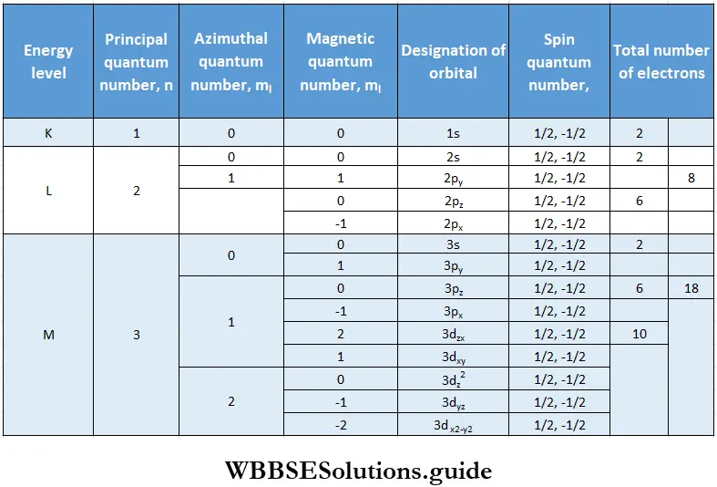
1. The principal quantum number n is a positive integer with values 1,2,3,— It determines the size of the orbital or electron cloud. In other words, it tells us what the average distance of the electron from the nucleus is. Orbitals with the same principal quantum number belong to the same shell. These shells are called K(n = 1), L (n = 2), M(n = 3), N(n = 4), etc.
2. It also defines the energy of an electron in a particular orbital. Each orbital is associated with a definite amount of energy is given by
⇒ \(E_n=-\frac{2 \pi^2 Z^2 e^4 m k^2}{n^2 h^2}\)
“Quantum Mechanical Model, orbitals, quantum numbers, and probability distribution, WBCHSE syllabus”
This expression is similar to the one obtained for Bohr orbits. E changes with n. Energy increases as n increases, or as the electron moves farther from the nucleus.
3. The principal quantum number also determines the maximum number of electrons that can be accommodated in a shell, which is 2n2. Thus, when n = 2 the maximum number of electrons is 2; when n = 2, the maximum number of electrons is 8, and so on. There is, however, an upper limit to the number of electrons that a shell (orbital) can accommodate. No shell has more than 32 electrons.
Azimuthal Quantum Number (l)
1. This is also called the orbital angular momentum or subsidiary quantum number because it determines the angular momentum of an electron in a particular orbital. If l is the azimuthal quantum number of an electron, its angular momentum works out to \((h / 2 \pi) \sqrt{l(l+1)}\). The magnitude of the angular momentum changes discontinuously from one orbital to another, or the angular momentum can have only certain discrete values.
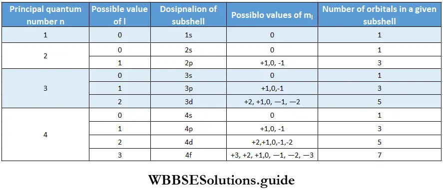
2. Each shell consists of one or more subshells, the number of subshells equals the value of n. The number of each subshell is the azimuthal quantum number, 1. The values that l may have for a given n are 0 and all positive integers up to n -1. Thus, for example, when n = 1, l can have only one value, i.e., 0; when n-2, l can be 0 or 1; when n = 3, l can be 0,1, or 2, and so on.
- Just as n denotes the shell an orbital (or an electron) belongs to, l stands for the subshell. The subshells are named s, p, d, and f. The letters s, p, d, and f originally were spectroscopic designations given to certain line spectra that correspond to atomic structure, s stood for sharp series, p for principal, d for diffuse, and f for fundamental series respectively. Now for higher values of n, say 5, l can attain values of 0,1,2, 3, and 4.
- The orbital for l = 4 is called g orbital. For higher l values the orbitals are named alphabetically (if onwards). However, these orbitals are too high in energy and not filled for known elements. The first shell has only one subshell designated Is (when n = 1, l = 0), the second shell has two (2s and 2p), the third shell has three (3s, 3p, 3d) and the fourth shell has four (4s, 4p, 4d, 4f) and so on. The maximum number of permissible subshells any shell has is four.
3. The value of 1 also determines the shape of an orbital. Different orbitals have different shapes. The s subshell (l = 0) is spherical, the p subshell (l = 1) is shaped like a dumbbell, the d subshell is shaped like double dumbbells and the f subshell has a rather complex shape.
4. The energy of a subshell depends on the value of l. The energies of subshells of the same principal shell increase as l increases in the following order.
s<p<d<f
This explains the fine lines (fine structure) observed in the hydrogen spectrum which Bohr’s model could not explain.
Magnetic Quantum Number (ml)
1. This is called the magnetic quantum number because it determines the behaviour of an electron under the influence of an external magnetic field. A revolving electron, possessing an angular momentum, has its own small magnetic field. When such an electron is placed in an external magnetic field, its own field gets oriented in a particular way, depending on the magnetic quantum number of the electron. Another way of saying this is that the magnetic quantum number determines the energies or the orientations of the orbitals of electrons in an external magnetic field.
“WBCHSE Class 11 Chemistry, quantum numbers, wave functions, and electron cloud model”
2. The magnetic quantum number determines the number of orientations of orbitals permitted in each subshell. The values that ml can have for a given l range from +l through 0 to -l, meaning that it can have 2l+1 values. If l = 1, for instance, the values of m} can be + 1,0 and -1.
3. The magnetic quantum number determinen the number of orientations possible in cacti subshcll or the number of orbitals that can be present in a subshell. Those orbitals have the same energy under normal circumstances, but not under the influence of an external magnetic field. This explains why spectral lines split into a number of fine lines when the source emitting the spectrum is placed in a magnetic field (Zeeman effect).
Spin Quantum Number (ms)
1. The spin quantum number was introduced by George Uhlenbeck and Samuel Goudsmit in 1925 to account for the spinning motion of an electron in Bohr’s model. The electron was thought to spin around its axis much the same way as planets do.
The spin quantum number (associated with Bohr’s model) could be +1/2 or -1/2 depending on whether the electron rotated clockwise or anticlockwise about its axis.
An electron in the quantum mechanical model also has a spin quantum number but it is not associated with the direction of axial rotation. It is a characteristic of the electron which determines its magnetic behaviour.
The two possible values of the spin quantum number, called up-spin and down-spin, are symbolically represented as ↑ and ↓. The values of the spin quantum number are independent of the values of the other three quantum numbers.
2. The spin quantum number is connected with the magnetic properties of the atom or the element. There is a simple explanation for this. An electron, as we have just discussed, is like a small magnet with a magnetic field of its own and a definite magnetic moment. (You will read more about this later.)
- Magnetic moment is a vector quantity and if an orbital contains two electrons, their magnetic moments are directed in opposite directions. (You will read in the next section that an orbital can have at most two electrons and they must have opposite spins.) The resultant of the oppositely directed magnetic moments is zero.
- Thus, if all the orbitals of an atom are filled, the net magnetic moment of the atom is zero. The magnetic properties of a substance depend on the magnetic moments of its atoms and molecules. If the net magnetic moment of the atoms of a substance is zero, the substance is diamagnetic If, on the other hand, the atoms of a substance contain half-filled orbitals, the net magnetic moment of the atoms is not zero and the substance is paramagnetic**.
The Pauli Exclusion Principle
By now you know that an electron in an orbital is defined by four quantum numbers, much as you are recognized by your name and address. However, two people from two different families can have the same name, but not the same address.
Similarly, two electrons in an atom cannot have the same set of quantum numbers. This principle was first put forward by the Austrian-Swiss physicist Wolfgang Pauli, who was awarded the Nobel Prize in Physics in 1945.
According to the principle, “No two electrons in an atom can have the same values for all the four quantum numbers,” because if one electron in an atom has a particular set of quantum numbers, all other electrons are excluded from having the same set of quantum numbers.
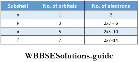
- This rule implies that an orbital can at the most have two electrons and the two electrons must have different spin quantum numbers. This is because electrons belonging to the same orbital must have the same values of n, l, and ml, so the only quantum number that can be different is ms, which can have only two values, which means that an orbital can have only two electrons in order not to violate Pauli’s rule.
- Take the 2s orbital, for example. All the electrons in this orbital have n = 2, l = 0, and mt = 0. The only variation possible is in the value of ms, so the 2s orbital can only accommodate two electrons, one with an up-spin (↑) and one with a down-spin (↓). Pauli’s rule makes it possible to calculate the maximum number of electrons that a subshell can accommodate.
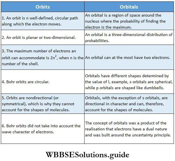
Now that you have a clear idea of orbitals in the quantum mechanical model of the atom, it would be worthwhile to enumerate the differences between the Bohr orbits and quantum mechanical orbitals.
Example 1. An electron is in 4d orbital. What are the possible values of n, l, ms, and ms for the electron.
Solution:
Given
An electron is in 4d orbital.
Since the orbital is 4d, n = 4 and l = 2.
ml can have values from -l to +l.
∴ ms =-2, -1,0,1,2.
ms = ±1/2(for each ml value).
“Quantum Mechanical Model of the Atom, principles, equations, and atomic structure, WBCHSE notes”
Example 2. Which of the following sets of quantum numbers is are not permitted?
- n=3, 1 = 3, m,=-2, ms = -1/2
- it =4, 1=3, mi = -3, ms = 1/2
- n =2, 1 = 0, m, =0, ms =0
- n=0, 1 = 0, mI =0, ms = -1/2
- n= 6, 1 = 4, m,=-2, ms = +1/2
Solution:
- Not permitted as l can take values from 0 to n – 1. l cannot be equal to n.
- Permitted.
- Not permitted as ms cannot be 0. It can be ± 1/2
- Not permitted as n cannot be 0.
- Permitted.
Example 3. Which of these orbitals are not possible? Give reasons to your answer. 1p, 2d, 3s, 4f, 3f
Solution:
lp is not possible as for n = 1, l = 0, therefore we can have only an s orbital.
2d is not possible because for n = 2, l = 0 and 1 and the corresponding orbitals are 2s and 2p.
3f is not possible because for n =3,1 = 0,1,2 and the permitted orbitals are 3s, 3p, 3d.
Example 4. Using s,p,d, and f notations, describe the orbital with the following quantum numbers:
- n = 2, l =0
- n =3,1 =2
- n =4,1 =3
- n=5,l = 4.
Solution:
- 2s
- 3d
- 4f and
- 5g
Shapes of orbitals: The orbitals of an atom have characteristic shapes. Imagine an electron in motion around the nucleus. The solutions of the Schrodinger equation for this electron cannot predict its exact location at any instant but it can give the probability of finding the electron in a certain location.
The probability distribution for an electron in the Is orbital could be likened to the holes in a rifle target of a good shooter.
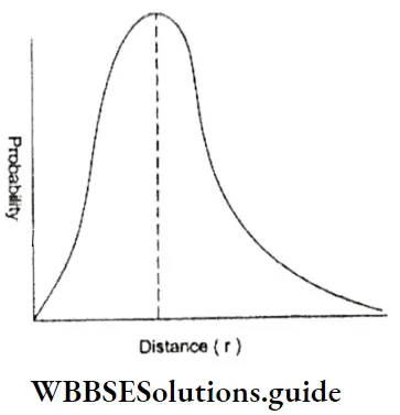
- The probability would be high (many holes) near the centre and decrease (fewer holes) as the distance from the centre (target) increases. Likewise, an electron is found, at any instant, with a higher probability closer to the nucleus than at a distance farther away. One way of representing this is as shown in Figure.
- This plot of probability versus distance takes into account two dimensions.
- An atomic orbital is that three-dimensional region in space where the probability of finding the electron is maximum. The shape of an orbital is defined as the surface enclosing 90% of the probability of finding the electron.
As stated earlier the square of the wave function, i.e., \(|\psi|^2\) at a point in an atom is a measure of the probability density at that point. The probability density \(|\psi|^2\) is not uniform in an atom.
It never becomes zero. To find out the shape of an atomic orbital, we draw the shapes based on the values of \(|\psi|^2\) in an atom.
- These most probable regions of finding electrons represent shapes of the orbitals and are called boundary surface diagrams. We cannot draw a boundary surface diagram in which the probability of finding an electron is 100% as \(|\psi|^2\) is never zero at any finite distance from the nucleus. In other words, it is not possible to draw a boundary surface diagram of a rigid size in which the probability of finding the electron is 100%.
Probability distribution curves: The plot of probability, i.e., \(|\psi|^2\) versus distance from the nucleus is called a probability distribution curve. Different orbitals are characterised by different probability distribution curves. The plot of the total probability density gives a boundary surface diagram and it indicates the shape of an orbital.
The wave function \(|\psi|^2\) of an electron can be divided into the radial part (dependent on the quantum numbers— n,l) and the angular part (dependent on the quantum numbers—l,ml) so that
⇒ \(\Psi=\underset{\text { radial angular }}{R} \underset{ }{\Phi}\)
Thus the wave function is split into two parts—radial and angular—which are solved separately.
Plots of radial wave function (R): The plots of R against r for 1s, 2s, and 2p orbitals are shown.
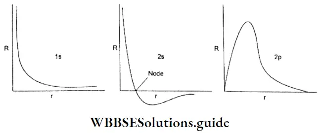
In all the cases R > 0 as r → ∞. In the 2s radial function, there is a node (region of zero probability). In general, ns orbitals have (n -1) nodes and tip orbitals have (n – 2) nodes. At a node, the sign of R changes.
Plot of radial probability density (R2) As you can see in Figure, for s orbitals the maximum electron density is close to the nucleus whereas for p orbital the electron density at the nucleus is zero.
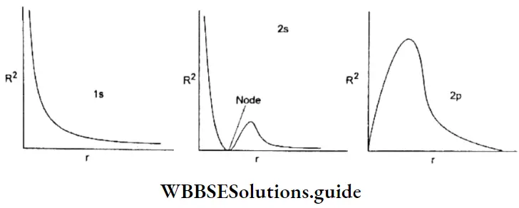
Plot of radial probability function: The plot of R2 against r gives the probability density of finding an electron at a distance r from the nucleus.
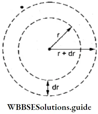
Atoms are considered to be spherical in shape. Let us consider the space around the nucleus to be divided into a large number of thin concentric spherical shells of thickness dr. Consider one of these shells with inner radius r.
The volume of such a shell is given by
dV = \(\frac{4}{3} \pi(r+d r)^3-\frac{4}{3} \pi r^3\)
Neglecting very small terms like dr2 and dr3, dV = 4πr2dr
The probability of finding an electron within this small radial shell is called the radial probability density function and is equal to 4πr2R2. A plot of the radial probability density function against the distance is called the radial probability distribution curve and gives the probability of finding an electron at a distance r from the nucleus.
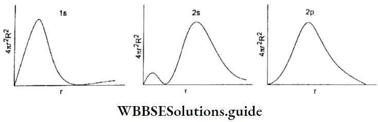
Interpretation of radial probability distribution curve: 1s orbital The probability of finding an electron at the nucleus is zero. This is significant as plots of R and R2 against r indicate that the maximum probability of finding an electron is at the nucleus, which is not true.
“WBCHSE Class 11, chemistry notes, on Quantum Model, Heisenberg Uncertainty Principle, and Schrödinger wave equation”
- The probability increases up to a point and then decreases. The maximum in the curve corresponds to the distance at which the probability of finding an electron is the maximum. This is called the radius of maximum probability.
- The curve indicates that the maximum probability of finding the electron of an atom is at the radius of maximum probability but does not rule out the fact that the electron may be at any other distance. This is in sharp contrast to the Bohr model in which the electron is restricted to a particular distance from the nucleus.
2s and 2p orbitals The curve for the 2s orbital has two maxima and a lldde (region of zero probability) between the two maxima, lire distance of maximum probability for a 2p electron is slightly less than that for a 2s electron.
- But the additional maximum in tire 2s curve is very significant. It indicates that a 2s electron in contrast to a 2p electron spends some time nearer the nucleus. It has greater penetration power and is more tightly held than a 2p electron. Hence a 2s electron is more stable and has lower energy than a 2p electron.
- As stated earlier the total wave function is made up of both radial and angular functions. It is difficult to picture angular functions but easier to visualise the probability density function. This can be done by representing the probability density by the density of shading Irt a diagram. A simpler method is to show only the boundary surface, the solid shape that contains about 90 pet cent t)f the electron probability.
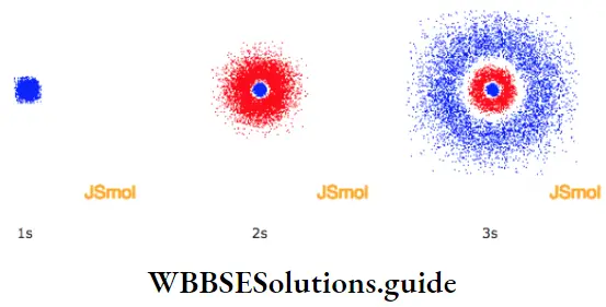
Boundary surfaces: For an s orbital, l = 0, so m1 = 0. This means that this orbital can have only one orientation about the nucleus; this will be possible only if the s orbital has the shape of a sphere.
The sphere is called the boundary surface, of the orbital. The s orbitals of higher energy levels are also spherical, but they have spherical shells within them where the probability is zero. These regions are called nodal surfaces or nodes or radial nodes. The 2s orbital has one node and the 3s orbital has two nodes. In general the 11s orbital has (n -1) nodes. The size and energy of the s orbitals increase with the value of n, i.e… Is < 2s < 3s ….
- We hope the question “How does an electron move from one probable region (orbital) to another when it is not allowed to be at the node (zero probability)?” is not bothering you. If it is, focus on the wavelike nature of the electron. In fact, nodes are an intrinsic property of waves.
- Apart from s orbitals, all other types of orbitals (l ≠ 0) have complicated boundary surfaces. The probability plots for a p orbital show three double-lobed or dumbbell-shaped orbitals oriented along each of the three mutually perpendicular axes.
- The two lobes in each orbital are separated by a nodal plane. There is zero probability density for electrons at this plane. Since the plane cuts through the nucleus, the probability of finding an electron at the nucleus is zero.
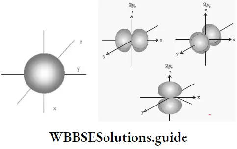
For p orbital, l = 1 and ml = -1, 0, +1, Consequently there are three orientations for the p orbitals. The size and energy of p orbital increases with n. Also as n increases, the p orbitals become bigger (as in the case of s orbitals) and show a complex radial nodal structure.
“Quantum Mechanical Model, significance of orbitals, and energy levels, WBCHSE syllabus”
- Generally speaking, the np orbital has (n- 2) radial nodes. For the same value of u, the three p orbitals have the same energy. Such orbitals, with the same energy, are called degenerate orbitals. When an external magnetic or electric field is applied these three orbitals get oriented differently and are no longer degenerate, (This explains the Zeeman effect.)
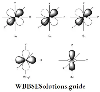
- Starting with the third principal energy level, one can have d orbitals. For d orbitals, l = 2 and ml = -2,-1,0,1- 1, + 2, Thus there are five degenerate d orbitals whose shapes are shown in Figure.
- The dxy, dxz, and dyz orbitals are alike except for the plane of their orientation and point between the two Cartesian axes. The \(\mathrm{d}_{x^2-y^2}\)orbital is like the dxy orbital except that it is rotated through 45° around the z axis and consists of a doughnut-scaped ring and dumbbell-shaped lobes.
- The \(\mathrm{d}_{z^2}\) orbital is symmetrical around the z axis. The probability density function of np and nd orbitals is zero at certain planes depending on the orientation of the orbital. The p and d orbitals are not spherically symmetrical. For the p7 orbital, there is no probability of finding the electron in the xy plane and this is a nodal plane. This is called an angular node and the number of angular nodes is given by l. Thus the p orbital has one angular node and the d orbital has two.